Twitter bot

I was talking with a friend about social networks when he mentioned that it wasn’t worth his time to invest on podcasts. He said that I looked up his twitter account, that that’s more useful for him. This reminded me that I haven’t used these wonderful tools about twitter nor had I the motivation for analyzing time serie data.

This blogpost is my attempt to find how this user uses some kind of automated mechanism to publish.

library("rtweet")
user_tweets <- get_timeline(user, n = 180000, type = "mixed", 
                            include_rts = TRUE)

Now that we have the tweets we can look if he is a bot:

library("tweetbotornot") # from mkearney/tweetbotornot
# you might need to install this specific version of textfeatures:
# devtools::install_version('textfeatures', version='0.2.0')
botornot(user_tweets)

## ↪ Counting features in text...
## ↪ Sentiment analysis...
## ↪ Parts of speech...
## ↪ Word dimensions started
## ✔ Job's done!

## # A tibble: 1 x 3
##   screen_name    user_id   prob_bot
##   <chr>          <chr>        <dbl>
## 1 josemariasiota 288661791    0.386

It gives a very high probability.

We can visualize them with:

library("ggplot2")
ts_plot(user_tweets, "weeks") +
  theme_bw() +
  labs(title = "Tweets by @josemariasiota",
       subtitle = "Grouped by week", x = NULL, y = "tweets")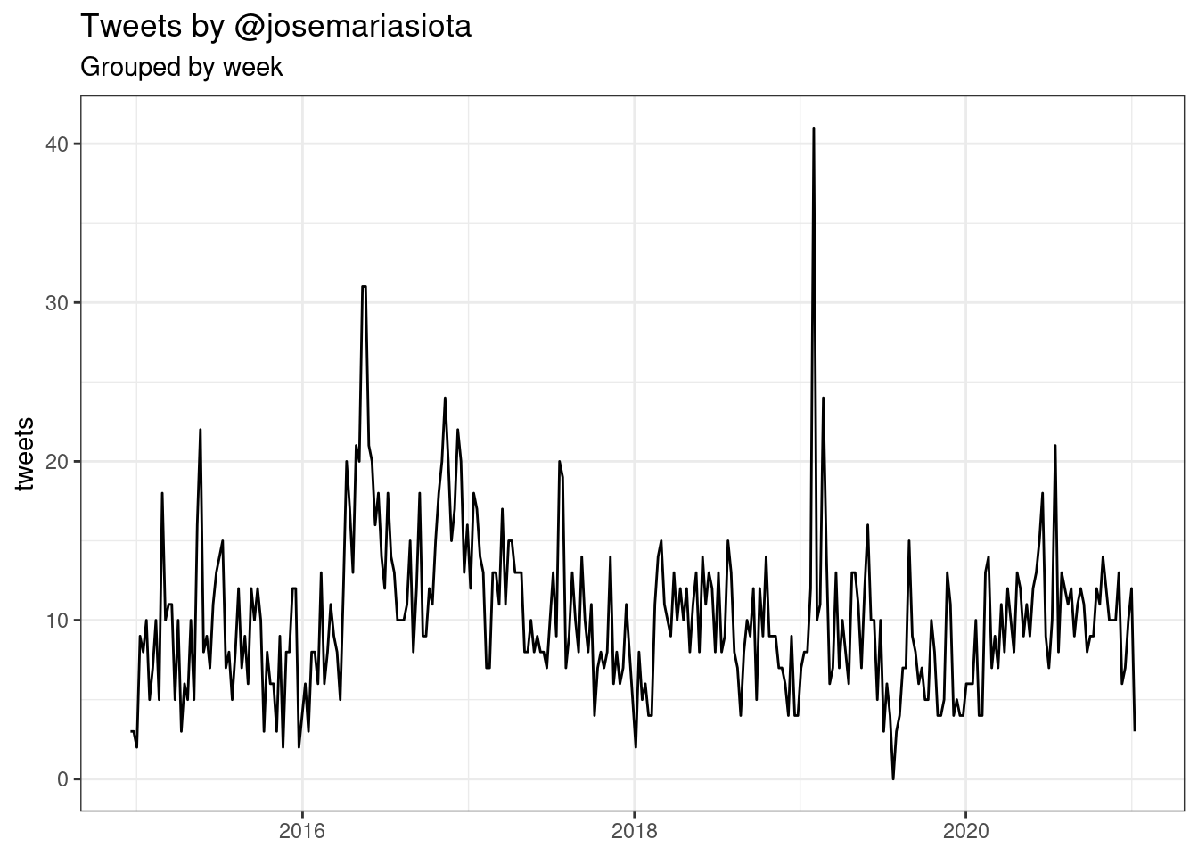

We can group the tweets by the source of them, if interactive or using some other service:

library("dplyr")

## 
## Attaching package: 'dplyr'

## The following objects are masked from 'package:stats':
## 
##     filter, lag

## The following objects are masked from 'package:base':
## 
##     intersect, setdiff, setequal, union

count(user_tweets, source, sort = TRUE)

## # A tibble: 9 x 2
##   source                               n
##   <chr>                            <int>
## 1 dlvr.it                           1738
## 2 twitterfeed                        676
## 3 Twitter Web Client                 553
## 4 Twitter Web App                    149
## 5 Twitter for iPhone                  78
## 6 Twitter for Advertisers (legacy)    21
## 7 Hootsuite                           13
## 8 Twitter for iPad                     2
## 9 Twitter for Websites                 2

user <- user_tweets %>% 
  mutate(source = case_when(
    grepl(" for | on | Web ", source) ~ "direct",
    TRUE ~ source
  ))

user %>% 
  count(source, sort = TRUE)

## # A tibble: 4 x 2
##   source          n
##   <chr>       <int>
## 1 dlvr.it      1738
## 2 direct        805
## 3 twitterfeed   676
## 4 Hootsuite      13

user <- user %>% 
  mutate(reply = case_when(
    is.na(reply_to_status_id) ~  "content?",
    TRUE ~ "reply"))
user %>% 
  count(reply, source, sort = TRUE)

## # A tibble: 5 x 3
##   reply    source          n
##   <chr>    <chr>       <int>
## 1 content? dlvr.it      1738
## 2 content? direct        731
## 3 content? twitterfeed   676
## 4 reply    direct         74
## 5 content? Hootsuite      13

library("stringr")
user <- user %>% 
  mutate(link = str_extract(text, "https?://.+\\b"),
         n_link = str_count(text, "https?://"),
         n_users = str_count(text, "@[:alnum:]+\\b"),
         n_hashtags = str_count(text, "#[:alnum:]+\\b"),
         via = str_count(text, "\\bvia\\b"))
user %>% count(n_link, reply, sort = TRUE)

## # A tibble: 7 x 3
##   n_link reply        n
##    <int> <chr>    <int>
## 1      1 content?  2508
## 2      2 content?   629
## 3      0 reply       57
## 4      0 content?    14
## 5      1 reply       14
## 6      3 content?     7
## 7      2 reply        3

user %>% 
  group_by(lang, source) %>% 
  summarise(n = n(), n_link = sum(n_link), n_users = sum(n_users), n_hashtags = sum(n_hashtags)) %>% 
  arrange(-n) %>% 
  ggplot() +
  geom_point(aes(lang, source, size = n)) +
  theme_bw()

## `summarise()` regrouping output by 'lang' (override with `.groups` argument)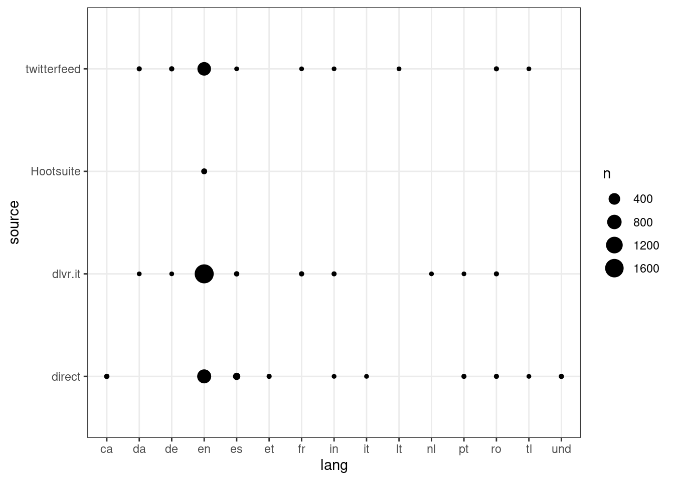

We can see that depending on the service there are some languages that are not used.

We can visualize the tweets as they happen with:

user %>% 
  mutate(hms = hms::as_hms(created_at),
         d = as.Date(created_at)) %>% 
  ggplot(aes(d, hms, col = source, shape = reply)) +
  geom_point() +
  theme_bw() +
  labs(y = "Hour", x = "Date", title = "Tweets") +
  scale_x_date(date_breaks = "1 year", date_labels = "%Y", 
               expand = c(0.01, 0)) +
  scale_y_time(labels = function(x) strftime(x, "%H"),
               breaks = hms::hms(seq(0, 24, 1)*60*60), expand = c(0.01, 0))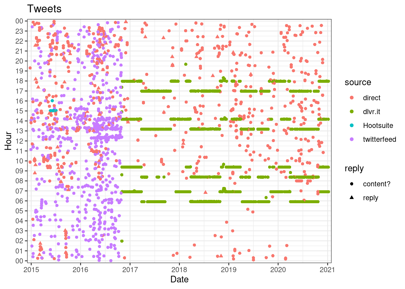

We can clearly see a change on the end of 2016, I will focus on that point forward.

A package that got my attention on twitter was anomalize which search for anomalies on time series of data. I hope that using this algorithm it will find when the data is not automated

library("anomalize")

## ══ Use anomalize to improve your Forecasts by 50%! ═════════════════════════════
## Business Science offers a 1-hour course - Lab #18: Time Series Anomaly Detection!
## </> Learn more at: https://university.business-science.io/p/learning-labs-pro </>

The excellent guide at their website is easy to understand and follow

user <- user %>% 
  filter(created_at > as.Date("2016-11-01")) %>% 
  arrange(created_at) %>% 
  time_decompose(created_at, method = "stl", merge = TRUE, message = TRUE) 

## Warning in mask$eval_all_filter(dots, env_filter): Incompatible methods
## ("Ops.POSIXt", "Ops.Date") for ">"

## Converting from tbl_df to tbl_time.
## Auto-index message: index = created_at

## frequency = 2 hours

## trend = 42.5 hours

## Registered S3 method overwritten by 'quantmod':
##   method            from
##   as.zoo.data.frame zoo

user %>% 
  filter(created_at > as.Date("2016-11-01")) %>% 
  anomalize(remainder, method = "iqr") %>%
  time_recompose() %>%
  # Anomaly Visualization
  plot_anomalies(time_recomposed = TRUE, ncol = 3, alpha_dots = 0.25) +
  labs(title = "User anomalies", 
       subtitle = "STL + IQR Methods", 
       x = "Time")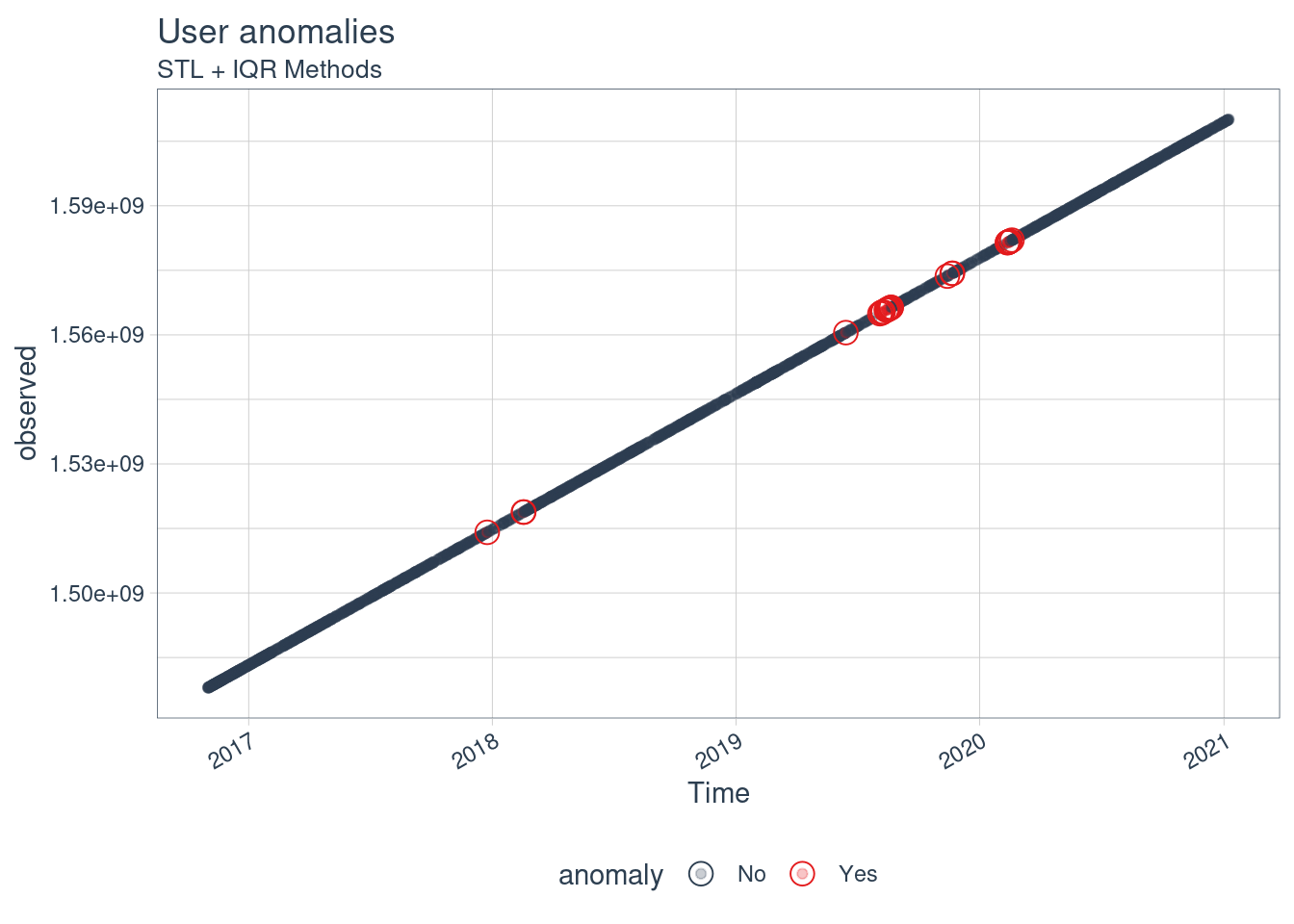 

user %>% 
  filter(created_at > as.Date("2016-11-01")) %>% 
  anomalize(remainder, method = "iqr") %>%
  plot_anomaly_decomposition() +
  labs(title = "Decomposition of Anomalized Lubridate Downloads")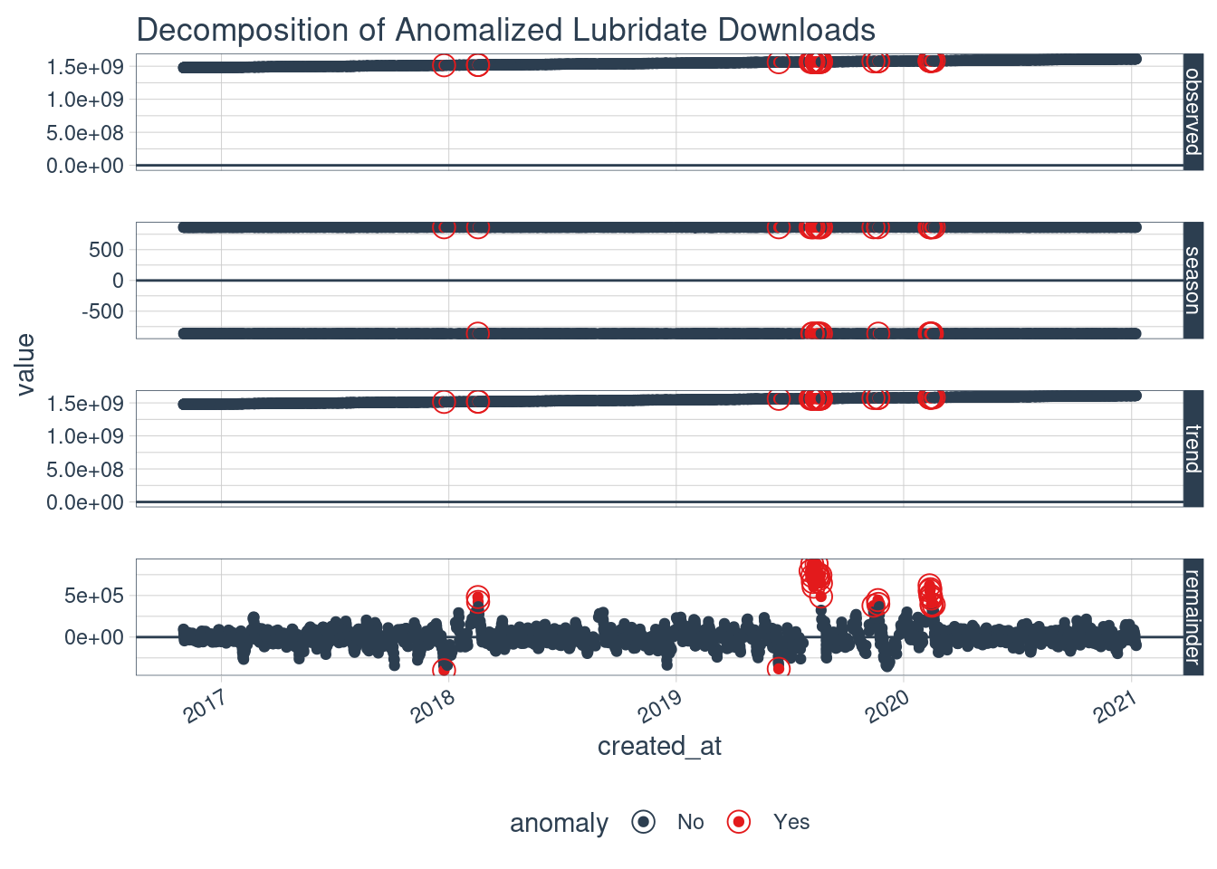

We can clearly see some tendencies on the tweeting so it is automated, since then. We can further check it with:

user %>% 
  filter(created_at > as.Date("2016-11-01")) %>% 
  botornot()

## ↪ Counting features in text...
## ↪ Sentiment analysis...
## ↪ Parts of speech...
## ↪ Word dimensions started
## ✔ Job's done!

## # A tibble: 1 x 3
##   screen_name    user_id   prob_bot
##   <chr>          <chr>        <dbl>
## 1 josemariasiota 288661791    0.469