Consumption of gasoline by our car
Does our car burns more gasoline now than on the first year?
Introduction
For years my dad has been taking the notes of the gas stations and annotating the km done by the car until that moment and the km since last stop to refill.
Now, he suspects that the car is not as efficient as it was so he want to check the gasoline consumption.
The data
knitr::opts_chunk$set(collapse = TRUE)I had to manually annotate the data, but I uploaded here:
library("here")
## here() starts at /home/lluis/Documents/Projects/blogR
raw_data <- read.csv(here("static", "gasolina.csv"))
It is tidy but real data; some errors, missing values are present. I start with a visualization:
library("ggplot2")
library("dplyr")
##
## Attaching package: 'dplyr'
## The following objects are masked from 'package:stats':
##
##     filter, lag
## The following objects are masked from 'package:base':
##
##     intersect, setdiff, setequal, union
library("lubridate")
##
## Attaching package: 'lubridate'
## The following objects are masked from 'package:base':
##
##     date, intersect, setdiff, union
clean_data <- raw_data %>%
  mutate(Date = dmy(Date)) %>%
  arrange(Date)

ggplot(clean_data) +
  geom_point(aes(Date, total_km, size = L)) +
  theme_bw()
## Warning: Removed 9 rows containing missing values (geom_point).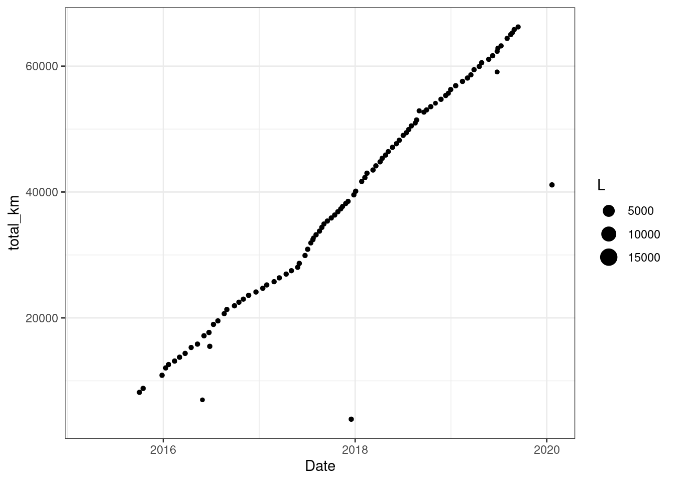
There are some values that are plain wrong, all of a sudden the car had less kilometers! Also we can see that there are some unit with more than 15000 Liters on the tank! We can check for other inconsistences.
summary(clean_data)
##       Date               Last_km          total_km           L
##  Min.   :2015-03-20   Min.   : 180.0   Min.   : 3906   Min.   :   11.95
##  1st Qu.:2016-11-11   1st Qu.: 495.3   1st Qu.:24841   1st Qu.:   32.96
##  Median :2017-11-14   Median : 540.7   Median :39034   Median :   36.60
##  Mean   :2017-10-29   Mean   : 575.9   Mean   :38702   Mean   :  216.95
##  3rd Qu.:2018-09-25   3rd Qu.: 602.0   3rd Qu.:53009   3rd Qu.:   39.97
##  Max.   :2020-01-21   Max.   :4597.6   Max.   :66228   Max.   :19349.00
##                       NA's   :12       NA's   :9       NA's   :1
##      Price
##  Min.   :14.00
##  1st Qu.:38.17
##  Median :42.10
##  Mean   :40.07
##  3rd Qu.:44.90
##  Max.   :54.01
##
We can see on the summary that there is a data point at the the 2020. In reality is a bill that had no year, so it is corrected by lubridate to 2020.
On the positive side it seems like the tank is bigger than expected and it can have more than 40 liters. We need to check the manual, but this came as a suprise to my father.
Data cleaning
Checking the originally data (make bakups or store the original data!), I found that instead of 19349 Liters it has been 19.49 L and the other outliers are also my mistake typing.
clean_data$L[clean_data$L > 100] <- 19.49
clean_data$Date[clean_data$Date > "2020/01/01"] <- "2018/01/21"
clean_data$Last_km[clean_data$Last_km > 1000] <- 597.6
clean_data$total_km[clean_data$total_km < 20000 &
                   year(clean_data$Date) < 2018 &
                   year(clean_data$Date) > 2016 &
                   !is.na(clean_data$total_km)] <- 39065
clean_data$total_km[clean_data$total_km < 7000 &
                   year(clean_data$Date) >= 2016 &
                   !is.na(clean_data$total_km)] <- 16977
# A duplicate with a wrong date
clean_data <- clean_data[clean_data$Date != "2019/03/26", ]
clean_data$Date[clean_data$Date == "2019/06/26" &
                   clean_data$total_km < 60000] <- "2019/03/26"
clean_data$total_km[clean_data$Date == "2016/06/26"] <- 18450
clean_data$total_km[clean_data$Date == "2016/06/26"] <- 18450
clean_data <- arrange(clean_data, Date)
After this manual curration we can check the plot again
ggplot(clean_data) +
  geom_point(aes(Date, total_km, size = L)) +
  theme_bw()  +
  labs(y = "Km accumulated")
## Warning: Removed 8 rows containing missing values (geom_point).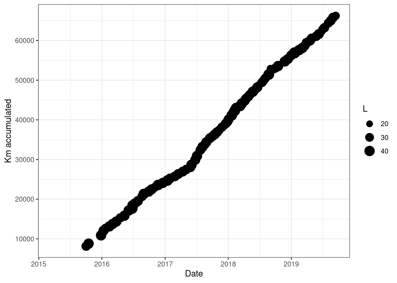
Now the plot is much better.
Insihgts
Efficiency
Now that the data has been corrected to the best of my hability we can start comparing liters and km:
cleaner_data <- clean_data %>%
  mutate(
    Last_km = round(Last_km),
    total_l = cumsum(coalesce(L, 0)),
    ratio = total_km/total_l
  )
In the last block we set up the data to make the comparison. Now we want to model the data, we will use broom:
library("broom")
model <- lm(total_km ~ total_l,
            data = filter(cleaner_data, !is.na(total_km)))

tidy(model)
## # A tibble: 2 x 5
##   term        estimate std.error statistic   p.value
##   <chr>          <dbl>     <dbl>     <dbl>     <dbl>
## 1 (Intercept)   6970.    65.6         106. 2.39e-101
## 2 total_l         16.0    0.0291      550. 9.13e-170
glance(model)
## # A tibble: 1 x 12
##   r.squared adj.r.squared sigma statistic   p.value    df logLik   AIC   BIC
##       <dbl>         <dbl> <dbl>     <dbl>     <dbl> <dbl>  <dbl> <dbl> <dbl>
## 1      1.00          1.00  293.   302741. 9.13e-170     1  -695. 1396. 1403.
## # … with 3 more variables: deviance <dbl>, df.residual <int>, nobs <int>
This means that every 15.9965533 km the car spends 1L, and it seems quite consistent over the years, but we missed around 6970 L before we started collecting data:
cleaner_data %>%
  filter(!is.na(total_km)) %>%
  ggplot(aes(total_l, total_km)) +
  geom_smooth(method = lm, col = "red") +
  geom_point() +
  theme_bw() +
  labs(x = "L accumulated", y = "Km accumulated")
## `geom_smooth()` using formula 'y ~ x'
Note that with 0 L we cannot have traveled. So, to get the real consumption we need to set it to 0:
model0 <- lm(total_km ~ 0 +total_l,
             data = filter(cleaner_data, !is.na(total_km)))

tidy(model0)
## # A tibble: 1 x 5
##   term    estimate std.error statistic   p.value
##   <chr>      <dbl>     <dbl>     <dbl>     <dbl>
## 1 total_l     18.8     0.142      132. 2.99e-111
Which results in a more efficient motor with close to 19km for each liter.
Now we can look if there are some years that it was worse. To do so we look at the residuals and the distribution of them:
augment(model) %>%
  cbind(filter(cleaner_data, !is.na(total_km))[ ,-c(3, 6)]) %>%
  ggplot() +
  geom_point(aes(Date, .resid)) +
  geom_smooth(aes(Date, .resid), method = "glm") +
  theme_minimal()
## `geom_smooth()` using formula 'y ~ x'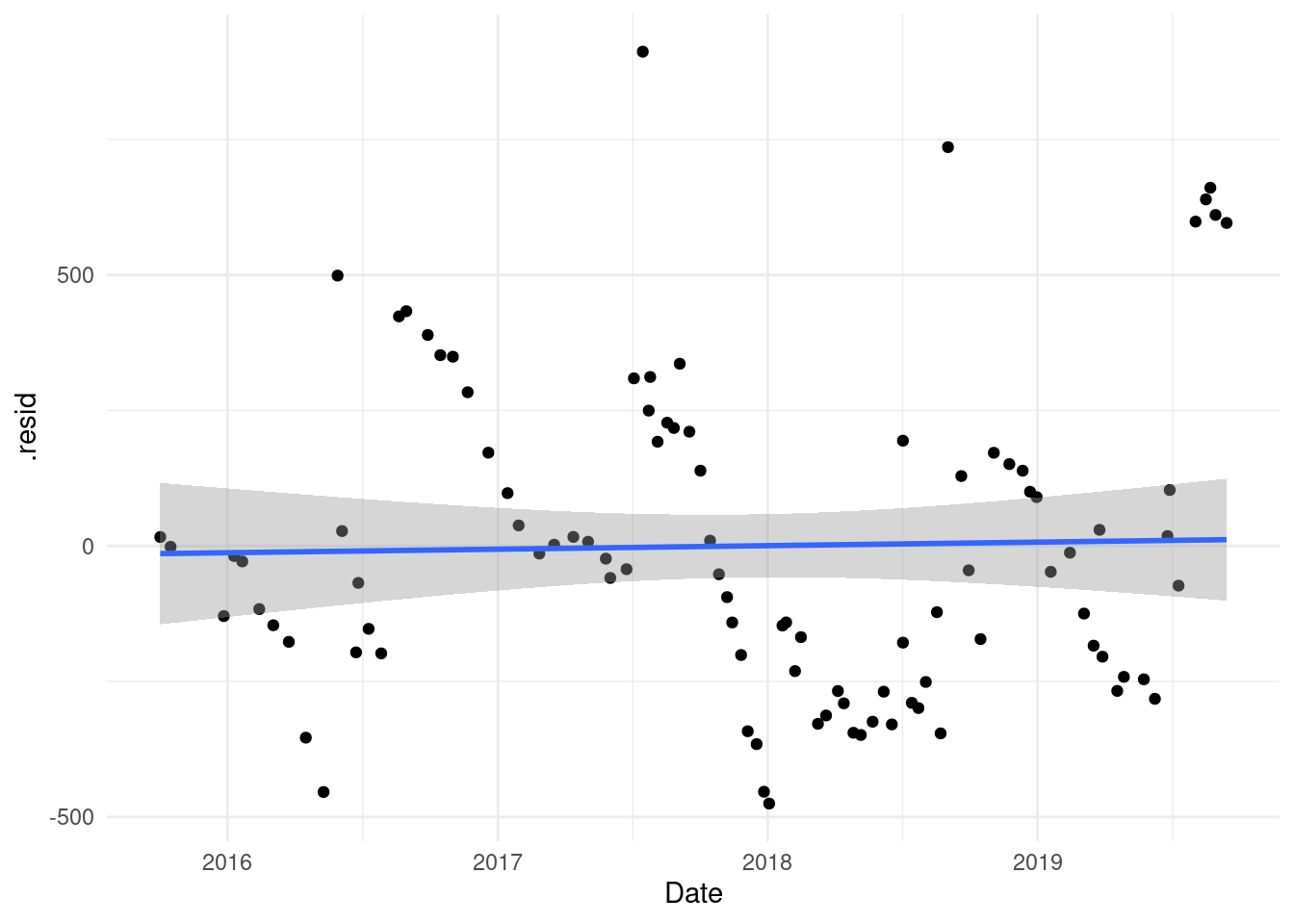
As we can see there is not a pattern here.
If the car were more efficient at the beginning we would see a trend that the residuals would increase.
But let’s check it :
augment(model) %>%
  cbind(filter(cleaner_data, !is.na(total_km))[ ,-c(3, 6)]) %>%
  lm(.resid ~ Date, data = .) %>%
  glance()
## # A tibble: 1 x 12
##   r.squared adj.r.squared sigma statistic p.value    df logLik   AIC   BIC
##       <dbl>         <dbl> <dbl>     <dbl>   <dbl> <dbl>  <dbl> <dbl> <dbl>
## 1  0.000581      -0.00983  293.    0.0558   0.814     1  -695. 1396. 1403.
## # … with 3 more variables: deviance <dbl>, df.residual <int>, nobs <int>
As we can see above we can’t say there is a linear tread to increased consumption with time.
Refills
Another interesting question is how many refills did we miss. We can first see how many km did it make with the last refill:
cleaner_data %>%
  ggplot() +
  geom_histogram(aes(Last_km)) +
  theme_bw()
## `stat_bin()` using `bins = 30`. Pick better value with `binwidth`.
## Warning: Removed 11 rows containing non-finite values (stat_bin).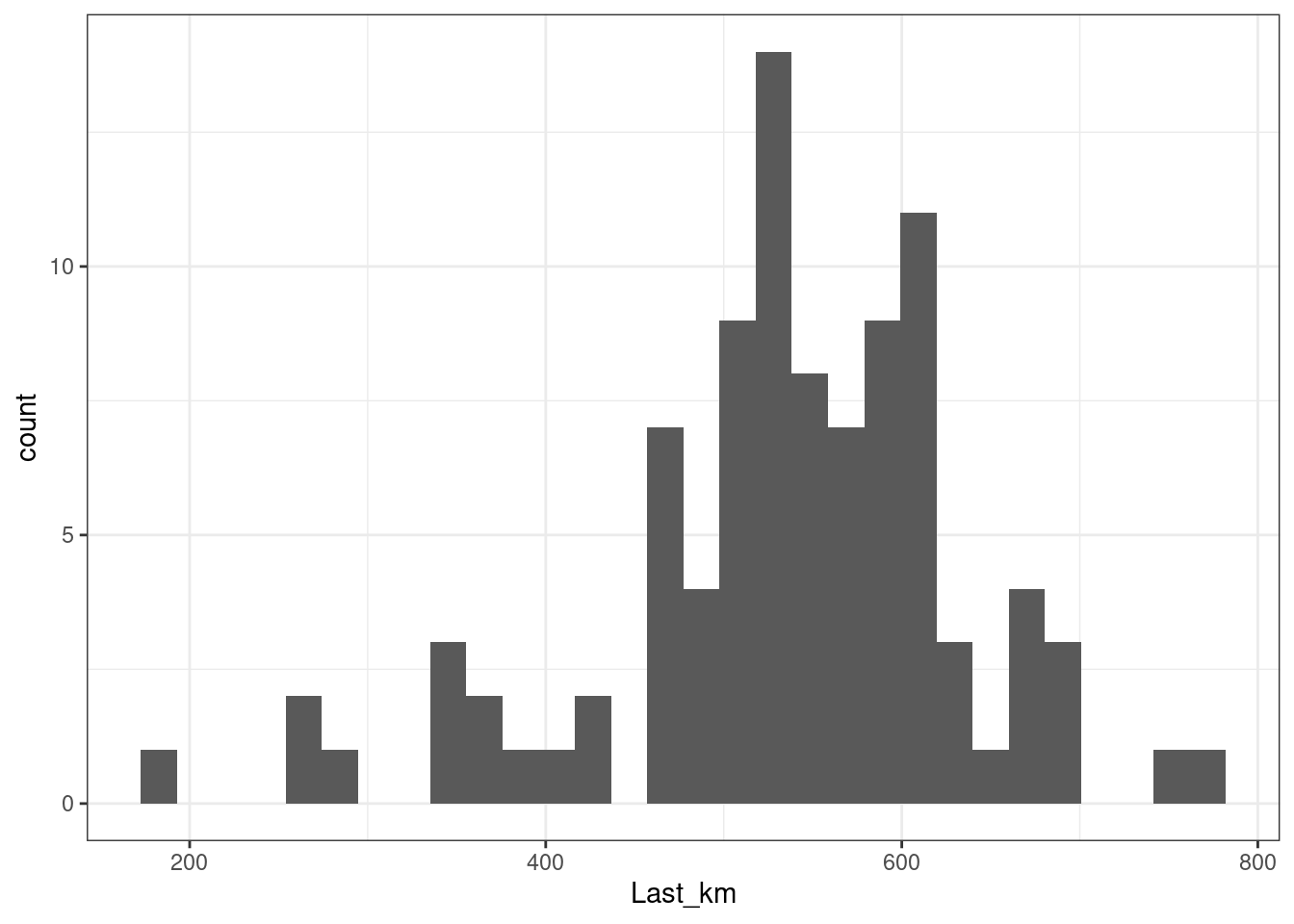
central_km <- cleaner_data %>%
  summarise(median = median(Last_km, na.rm = TRUE),
            mean = round(mean(Last_km, na.rm = TRUE)))
central_km
##   median mean
## 1    541  534
# Then we can divide the total
max(cleaner_data$total_km, na.rm = TRUE)/central_km[1, ]
##     median     mean
## 1 122.4177 124.0225
We can round this to 123 refills. So apparently we missed 17 refills. Or did I miss something here?
Let’s check how many refills are already missing from the data we have:
cleaner_data %>%
  mutate(
    cum_km = cumsum(coalesce(Last_km, 0)),
    km_at_last_refill = total_km - Last_km,
    diff = total_km - km_at_last_refill[-1],
    diff = if_else(is.na(diff), 0, diff),
    refills_missed = round(abs(diff)/median(Last_km, na.rm = TRUE))
  ) %>%
  summarise(total = sum(refills_missed))
## Warning: Problem with `mutate()` input `diff`.
## ℹ longer object length is not a multiple of shorter object length
## ℹ Input `diff` is `total_km - km_at_last_refill[-1]`.
## Warning in total_km - km_at_last_refill[-1]: longer object length is not a
## multiple of shorter object length
##   total
## 1     8
To that amount we need to add the first 8171 km that we don’t have information of the refills. But those are around 14, plus the one we already have come close to those 17 we estimated. The difference is because there have been some smaller refills.
Long and short distances
If we look at it as a time series, we might notice some jumps. This might be due to a long trip. We can see if we can extract if there are some anomalies on the serie:
library("anomalize")
## ══ Use anomalize to improve your Forecasts by 50%! ═════════════════════════════
## Business Science offers a 1-hour course - Lab #18: Time Series Anomaly Detection!
## </> Learn more at: https://university.business-science.io/p/learning-labs-pro </>
cleaner_data %>%
  filter(!is.na(total_km)) %>%
  as_tibble() %>%
  time_decompose(total_km, method = "stl") %>%
  anomalize(remainder, method = "iqr") %>%
  time_recompose() %>%
  plot_anomalies(time_recomposed = TRUE, ncol = 3, alpha_dots = 0.25) +
  labs(title = "Refill Anomalies", subtitle = "STL + IQR Methods")
## Converting from tbl_df to tbl_time.
## Auto-index message: index = Date
## frequency = 20 months
## trend = 20 months
## Registered S3 method overwritten by 'quantmod':
##   method            from
##   as.zoo.data.frame zoo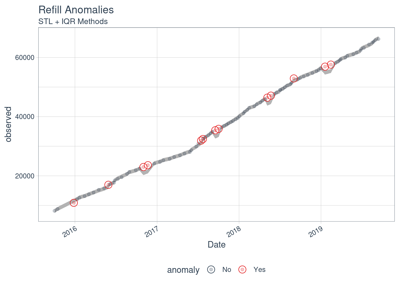
We can further explore if there is any anomaly:
cleaner_data %>%
  filter(!is.na(total_km)) %>%
  time_frequency(period = "auto")
## frequency = 20 months
## [1] 20
cleaner_data %>%
  filter(!is.na(total_km)) %>%
  time_trend(period = "auto")
## trend = 20 months
## [1] 20

al <- cleaner_data %>%
  filter(!is.na(total_l)) %>%
  as_tibble() %>%
  time_decompose(total_l, method = "stl", trend = "1 year", frequency = "1 months") %>%
  anomalize(remainder, method = "iqr") %>%
  plot_anomaly_decomposition() +
  labs(title = "total l")
## Converting from tbl_df to tbl_time.
## Auto-index message: index = Date
## frequency = 2 months
## trend = 22 months
ak <- cleaner_data %>%
  filter(!is.na(total_km)) %>%
  as_tibble() %>%
  time_decompose(total_km, method = "stl", trend = "1 year", frequency = "1 months") %>%
  anomalize(remainder, method = "iqr") %>%
  plot_anomaly_decomposition() +
  labs(title = "total km")
## Converting from tbl_df to tbl_time.
## Auto-index message: index = Date
## frequency = 2 months
## trend = 20 months

ar <- cleaner_data %>%
  filter(!is.na(ratio)) %>%
  as_tibble() %>%
  time_decompose(ratio, method = "stl") %>%
  anomalize(remainder, method = "iqr") %>%
  plot_anomaly_decomposition() +
  labs(title = "total km/l")
## Converting from tbl_df to tbl_time.
## Auto-index message: index = Date
## frequency = 20 months
## trend = 20 months
library("patchwork")
al + ak + plot_annotation(title = "Anomalies")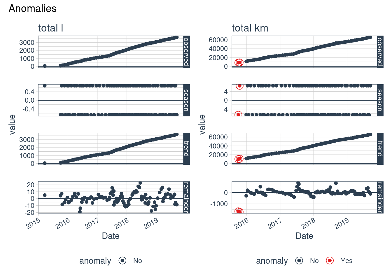
Conclusions
We can say that the car doesn’t need more gasoline for the same distance.
Usually there is a refill for every 550 km.
There aren’t notable anomalies, so the car makes the same trips usually.
References
Reproducibility
## ─ Session info ───────────────────────────────────────────────────────────────────────────────────────────────────────
##  setting  value
##  version  R version 4.0.1 (2020-06-06)
##  os       Ubuntu 20.04.1 LTS
##  system   x86_64, linux-gnu
##  ui       X11
##  language (EN)
##  collate  en_US.UTF-8
##  ctype    en_US.UTF-8
##  tz       Europe/Madrid
##  date     2021-01-08
##
## ─ Packages ───────────────────────────────────────────────────────────────────────────────────────────────────────────
##  package       * version    date       lib source
##  anomalize     * 0.2.2      2020-10-20 [1] CRAN (R 4.0.1)
##  assertthat      0.2.1      2019-03-21 [1] CRAN (R 4.0.1)
##  backports       1.2.1      2020-12-09 [1] CRAN (R 4.0.1)
##  blogdown        0.21.84    2021-01-07 [1] Github (rstudio/blogdown@c4fbb58)
##  bookdown        0.21       2020-10-13 [1] CRAN (R 4.0.1)
##  broom         * 0.7.3      2020-12-16 [1] CRAN (R 4.0.1)
##  class           7.3-17     2020-04-26 [1] CRAN (R 4.0.1)
##  cli             2.2.0      2020-11-20 [1] CRAN (R 4.0.1)
##  codetools       0.2-18     2020-11-04 [1] CRAN (R 4.0.1)
##  colorspace      2.0-0      2020-11-11 [1] CRAN (R 4.0.1)
##  crayon          1.3.4      2017-09-16 [1] CRAN (R 4.0.1)
##  curl            4.3        2019-12-02 [1] CRAN (R 4.0.1)
##  dials           0.0.9      2020-09-16 [1] CRAN (R 4.0.1)
##  DiceDesign      1.8-1      2019-07-31 [1] CRAN (R 4.0.1)
##  digest          0.6.27     2020-10-24 [1] CRAN (R 4.0.1)
##  dplyr         * 1.0.2      2020-08-18 [1] CRAN (R 4.0.1)
##  ellipsis        0.3.1      2020-05-15 [1] CRAN (R 4.0.1)
##  evaluate        0.14       2019-05-28 [1] CRAN (R 4.0.1)
##  fansi           0.4.1      2020-01-08 [1] CRAN (R 4.0.1)
##  farver          2.0.3      2020-01-16 [1] CRAN (R 4.0.1)
##  foreach         1.5.1      2020-10-15 [1] CRAN (R 4.0.1)
##  forecast        8.13       2020-09-12 [1] CRAN (R 4.0.1)
##  fracdiff        1.5-1      2020-01-24 [1] CRAN (R 4.0.1)
##  furrr           0.2.1      2020-10-21 [1] CRAN (R 4.0.1)
##  future          1.21.0     2020-12-10 [1] CRAN (R 4.0.1)
##  generics        0.1.0      2020-10-31 [1] CRAN (R 4.0.1)
##  ggplot2       * 3.3.2      2020-06-19 [1] CRAN (R 4.0.1)
##  globals         0.14.0     2020-11-22 [1] CRAN (R 4.0.1)
##  glue            1.4.2      2020-08-27 [1] CRAN (R 4.0.1)
##  gower           0.2.2      2020-06-23 [1] CRAN (R 4.0.1)
##  GPfit           1.0-8      2019-02-08 [1] CRAN (R 4.0.1)
##  gtable          0.3.0      2019-03-25 [1] CRAN (R 4.0.1)
##  here          * 1.0.1      2020-12-13 [1] CRAN (R 4.0.1)
##  hms             0.5.3      2020-01-08 [1] CRAN (R 4.0.1)
##  htmltools       0.5.0      2020-06-16 [1] CRAN (R 4.0.1)
##  httr            1.4.2      2020-07-20 [1] CRAN (R 4.0.1)
##  ipred           0.9-9      2019-04-28 [1] CRAN (R 4.0.1)
##  iterators       1.0.13     2020-10-15 [1] CRAN (R 4.0.1)
##  jsonlite        1.7.2      2020-12-09 [1] CRAN (R 4.0.1)
##  knitcitations * 1.0.10     2019-09-15 [1] CRAN (R 4.0.1)
##  knitr           1.30       2020-09-22 [1] CRAN (R 4.0.1)
##  labeling        0.4.2      2020-10-20 [1] CRAN (R 4.0.1)
##  lattice         0.20-41    2020-04-02 [1] CRAN (R 4.0.1)
##  lava            1.6.8.1    2020-11-04 [1] CRAN (R 4.0.1)
##  lhs             1.1.1      2020-10-05 [1] CRAN (R 4.0.1)
##  lifecycle       0.2.0      2020-03-06 [1] CRAN (R 4.0.1)
##  listenv         0.8.0      2019-12-05 [1] CRAN (R 4.0.1)
##  lmtest          0.9-38     2020-09-09 [1] CRAN (R 4.0.1)
##  lubridate     * 1.7.9.2    2020-11-13 [1] CRAN (R 4.0.1)
##  magrittr        2.0.1      2020-11-17 [1] CRAN (R 4.0.1)
##  MASS            7.3-53     2020-09-09 [1] CRAN (R 4.0.1)
##  Matrix          1.2-18     2019-11-27 [1] CRAN (R 4.0.1)
##  mgcv            1.8-33     2020-08-27 [1] CRAN (R 4.0.1)
##  munsell         0.5.0      2018-06-12 [1] CRAN (R 4.0.1)
##  nlme            3.1-151    2020-12-10 [1] CRAN (R 4.0.1)
##  nnet            7.3-14     2020-04-26 [1] CRAN (R 4.0.1)
##  parallelly      1.22.0     2020-12-13 [1] CRAN (R 4.0.1)
##  parsnip         0.1.4      2020-10-27 [1] CRAN (R 4.0.1)
##  patchwork     * 1.1.1      2020-12-17 [1] CRAN (R 4.0.1)
##  pillar          1.4.7      2020-11-20 [1] CRAN (R 4.0.1)
##  pkgconfig       2.0.3      2019-09-22 [1] CRAN (R 4.0.1)
##  plyr            1.8.6      2020-03-03 [1] CRAN (R 4.0.1)
##  pROC            1.16.2     2020-03-19 [1] CRAN (R 4.0.1)
##  prodlim         2019.11.13 2019-11-17 [1] CRAN (R 4.0.1)
##  purrr           0.3.4      2020-04-17 [1] CRAN (R 4.0.1)
##  quadprog        1.5-8      2019-11-20 [1] CRAN (R 4.0.1)
##  quantmod        0.4.18     2020-12-09 [1] CRAN (R 4.0.1)
##  R6              2.5.0      2020-10-28 [1] CRAN (R 4.0.1)
##  Rcpp            1.0.5      2020-07-06 [1] CRAN (R 4.0.1)
##  readr           1.4.0      2020-10-05 [1] CRAN (R 4.0.1)
##  recipes         0.1.15     2020-11-11 [1] CRAN (R 4.0.1)
##  RefManageR      1.3.0      2020-11-13 [1] CRAN (R 4.0.1)
##  rlang           0.4.10     2020-12-30 [1] CRAN (R 4.0.1)
##  rmarkdown       2.6        2020-12-14 [1] CRAN (R 4.0.1)
##  rpart           4.1-15     2019-04-12 [1] CRAN (R 4.0.1)
##  rprojroot       2.0.2      2020-11-15 [1] CRAN (R 4.0.1)
##  rsample         0.0.8      2020-09-23 [1] CRAN (R 4.0.1)
##  rstudioapi      0.13       2020-11-12 [1] CRAN (R 4.0.1)
##  scales          1.1.1      2020-05-11 [1] CRAN (R 4.0.1)
##  sessioninfo     1.1.1      2018-11-05 [1] CRAN (R 4.0.1)
##  stringi         1.5.3      2020-09-09 [1] CRAN (R 4.0.1)
##  stringr         1.4.0      2019-02-10 [1] CRAN (R 4.0.1)
##  survival        3.2-7      2020-09-28 [1] CRAN (R 4.0.1)
##  sweep           0.2.3      2020-07-10 [1] CRAN (R 4.0.1)
##  tibble          3.0.4      2020-10-12 [1] CRAN (R 4.0.1)
##  tibbletime      0.1.6      2020-07-21 [1] CRAN (R 4.0.1)
##  tidyr           1.1.2      2020-08-27 [1] CRAN (R 4.0.1)
##  tidyselect      1.1.0      2020-05-11 [1] CRAN (R 4.0.1)
##  timeDate        3043.102   2018-02-21 [1] CRAN (R 4.0.1)
##  timetk          2.6.0      2020-11-21 [1] CRAN (R 4.0.1)
##  tseries         0.10-48    2020-12-04 [1] CRAN (R 4.0.1)
##  TTR             0.24.2     2020-09-01 [1] CRAN (R 4.0.1)
##  tune            0.1.2      2020-11-17 [1] CRAN (R 4.0.1)
##  urca            1.3-0      2016-09-06 [1] CRAN (R 4.0.1)
##  utf8            1.1.4      2018-05-24 [1] CRAN (R 4.0.1)
##  vctrs           0.3.6      2020-12-17 [1] CRAN (R 4.0.1)
##  withr           2.3.0      2020-09-22 [1] CRAN (R 4.0.1)
##  workflows       0.2.1      2020-10-08 [1] CRAN (R 4.0.1)
##  xfun            0.20       2021-01-06 [1] CRAN (R 4.0.1)
##  xml2            1.3.2      2020-04-23 [1] CRAN (R 4.0.1)
##  xts             0.12.1     2020-09-09 [1] CRAN (R 4.0.1)
##  yaml            2.2.1      2020-02-01 [1] CRAN (R 4.0.1)
##  yardstick       0.0.7      2020-07-13 [1] CRAN (R 4.0.1)
##  zoo             1.8-8      2020-05-02 [1] CRAN (R 4.0.1)
##
## [1] /home/lluis/bin/R/4.0.1/lib/R/library